How fast can a HiWonder arm move?
I want my HiWonder arm to move between adjacent chessboard squares in 0.5 seconds, then make 30 complete F1–G1–F1 roundtrips in at most 65 seconds. The squares are 20 mm wide, and the pointer is commanded to hover 20 mm above the board.
The latest experiment completed all 30 roundtrips with passing modeled arrival checks, but took 67.56 seconds. Those original time targets were not achieved. I have accepted this timing for the next task: collecting motion across all 64 squares. The useful finding so far is that command scheduling, status polling and recording overhead account for a substantial part of the delay.
The specification gives an optimistic scale
HiWonder lists LX-225 speed as 0.20 seconds per 60 degrees at 7.4 V, and LX-15D speed as 0.22 seconds per 60 degrees. The xArm 1S product specification lists both servo types. I have not independently verified which model is installed at every joint on this bench.
The new 20 mm hover model needs approximately 43 base ticks between F1 and G1. At 0.24 degrees per tick, that is 10.32 degrees. Applying the two nominal servo speeds gives a speed-only scale of roughly 34–38 milliseconds for that rotation.
The loaded arm still has to accelerate, brake and settle. Gears, payload, internal servo control, power and communications add delay. The practical limit needs measurement; these specifications cannot establish that half a second is half of the physical limit.
For distance d, speed limit v and constant acceleration limit a, an ideal move that starts and finishes stationary takes at least:
2 * sqrt(d / a)    when d <= v*v/a
d/v + v/a         otherwise
That is a triangular or trapezoidal velocity profile. The loaded actuator acceleration limit remains unmeasured. The mathematical acceleration bound in the planner is a software setting.
Measure arrival, not just the requested duration
I am testing Castor on Atlas through its existing exclusive robot owner. The wrist fisheye and fixed table camera stay connected, and continuous recording retains the attempts. Private bench photographs remain private.
Position comes from measured servo ticks passed through a pinned geometric model. The current arrival check requires horizontal error within 2 mm, modeled height between 18 and 23 mm, and estimated horizontal speed at most 5 mm/s. A line fit through three distinct feedback sweeps estimates speed. Repeated status snapshots do not become extra measurements.
Those sweeps span at least 100 ms. With the current feedback cadence, three readings typically span about 250 ms. Joint timestamps are host receipt times, and readings within a sweep differ in time. These are modeled bench measurements; independent physical accuracy and the stricter final timing method still need qualification.
A separate one-second stationary diagnostic initially added a pause after each move. I removed that fixed dwell. Later tests also reuse real feedback seen during execution, rather than restarting the same arrival estimator after native completion. Every observation is retained, and stale or invalid readings reset the check.
What changed in the controller
An earlier Castor accuracy panel took median times of 34.3 seconds toward G1 and 28.3 seconds toward F1. It used small decisions and repeated short paths, at approximately 10 mm hover. That historical result is a scheduling clue, not a matched baseline for the new 20 mm experiment.
The new approach computes the destination and coordinated motion directly. A deterministic C++ trajectory calculator generates a smooth fifth-order reference:
q(u) = q0 + (q1-q0) * (10*u^3 - 15*u^4 + 6*u^5)
u = elapsed time / requested duration
Its peak reference speed is 1.875 * displacement / duration; peak reference acceleration is approximately 5.774 * displacement / duration^2. These describe the planned curve. The actual native owner and firmware determine its execution.
For row 1, holding the shoulder and elbow steady and solving base rotation plus wrist pitch worked better than repeatedly correcting several axes. A fresh A1–H1 traversal at a one-second requested profile passed all eight modeled endpoint checks without corrections. Earlier misses and start-binding rejections remain in the ledger.
I then reduced expensive dashboard polling. Normal pose and completion checks can read the owner’s atomically published status through its existing helper. Command admission, Stop, camera checks, lease checks and endpoint recovery still use the native control path. No second USB connection is opened.
Finally, I compared sampled references with one coordinated firmware-duration target. A single target sends all moving joints together. It does not claim that the firmware follows the fifth-order curve internally.
Ten trials per direction
These medians run from submission to verified arrival, including the applicable observation delay. Each row contains ten F1-to-G1 and ten G1-to-F1 trials. The client and observation method evolved between panels; they are successive engineering experiments rather than a controlled actuator comparison.
| Requested duration and client | Toward G1 | Toward F1 |
|---|---|---|
| 1.0 s, fixed dwell removed | 2.59 s | 2.01 s |
| 0.75 s, dashboard polling | 1.72 s | 2.33 s |
| 0.5 s, dashboard polling | 3.15 s | 1.93 s |
| 0.5 s, native observation | 1.27 s | 1.18 s |
| 0.4 s, single target and reused arrival history | 1.01 s | 1.10 s |
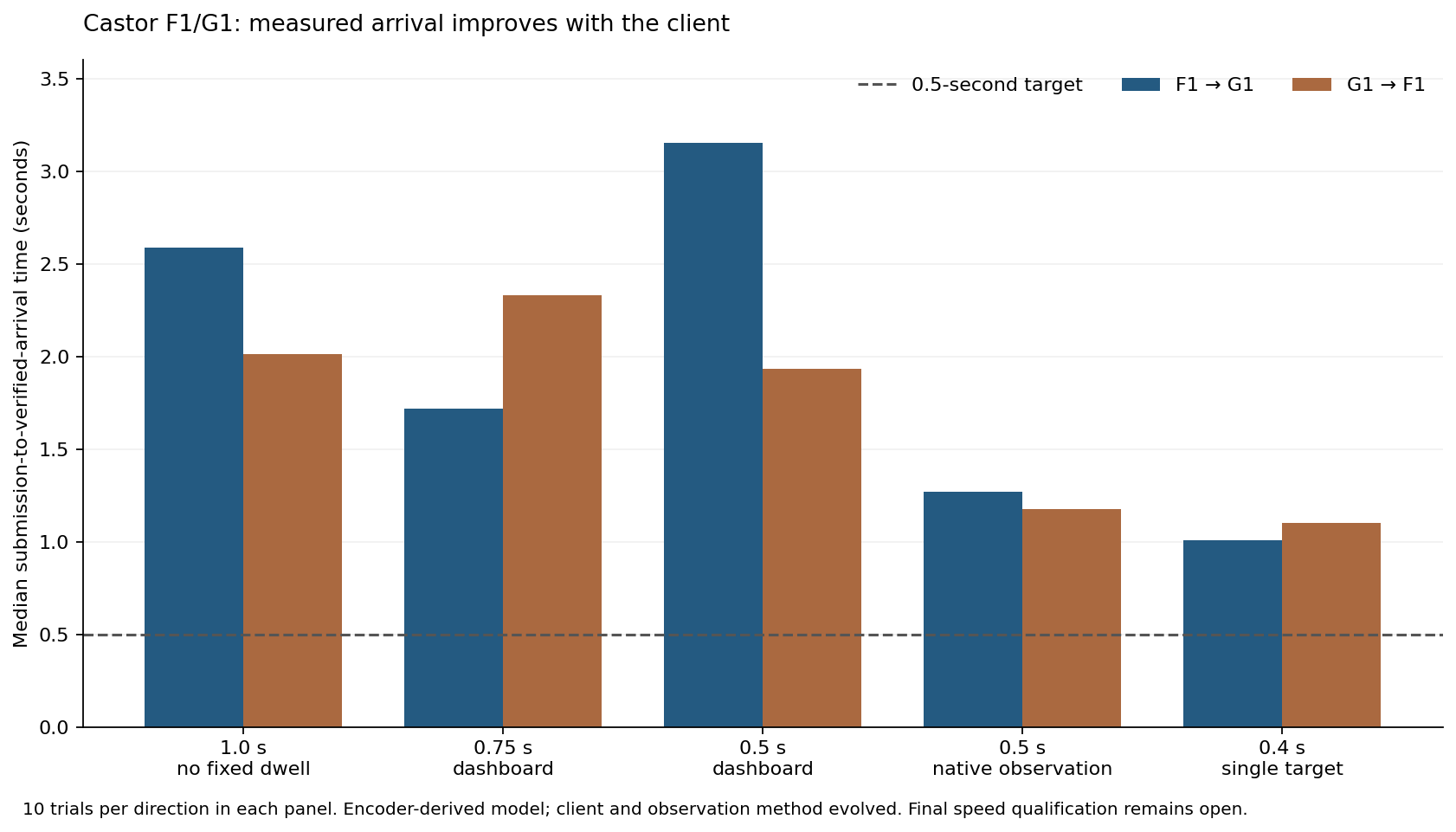
A shorter requested duration did not reliably make the full operation faster. The original 0.5-second panel had long delays despite passing its arrival checks. Reading native status reduced those delays, but native completion, recording readiness and admission still consume time.
Thirty full roundtrips
Each sustained run finished setup at F1 before starting the timer, then included all 60 legs and every between-leg gap.
| Fresh 30-roundtrip panel | Full elapsed time |
|---|---|
| 400 ms targets, growing result-file rewrites | 93.87 s |
| 400 ms targets, small durable checkpoints | 68.21 s |
| 375 ms targets, small durable checkpoints | 67.56 s |
All 60 modeled arrival checks passed in each panel. In the latest run, median verified arrival was 1.11 seconds toward G1 and 1.05 seconds toward F1; the worst legs took 1.39 and 1.25 seconds. No leg met the half-second requirement, and the total still exceeded 65 seconds.
The first run’s leg intervals totaled 86.75 seconds, with between-leg gaps adding 7.13 seconds. Those gaps grew as the experiment rewrote a larger result file. Native logs also recorded 23 dispatch deferrals across the new comparison runs because telemetry rate fell below recording-readiness requirements. Replacing full report rewrites with small durable checkpoints reduced contention. The complete trace is saved after recording ends, while native receipts and recording remain independent.
Angular speed and acceleration estimates
For the latest 375 ms panel, I calculated velocity from adjacent per-joint encoder receipts and acceleration from three successive readings. I skipped gaps over 200 ms and kept the original positions.
Across thirty trials per direction, the median per-trial peak interval speed of the base was approximately 32 degrees per second. Median three-point peak acceleration estimates were approximately 179–184 degrees per second squared. At the observed cadence, changing each of the three samples by one tick changes that acceleration estimate by as much as approximately 62 degrees per second squared.
That is a sensitivity calculation, not a confidence interval. Host receipt timing, potentiometer error and coarse sampling remain limitations. These estimates characterize the tested motion, not the maximum loaded actuator acceleration or its instantaneous peak.
Download all 60 latest sustained observations, the previous 400 ms checkpoint run, the retained 93.87-second run, angular motion estimates, and row-1 results. Raw recordings, native receipts and failed attempts have verified off-host copies. The separate experiment repository is hiwonder-speed-tests.
Motion data across all 64 squares
The controller now reaches every square. The farther rows need shoulder and elbow changes; row 1’s two-axis method alone cannot cover the board. The geometric planner prefers held posture where it fits, then solves additional joints when needed. Directional command compensation accounts for observed deadband, and endpoint checks still use raw measured joints.
There are now 685 recorded visits meeting the model and saved-frame checks across all 64 squares, with 10 to 12 visits per square. The ten-visits-per-square target is complete. Each data visit has a freshly persisted wrist frame, its hash and a causally aligned native joint sample. These labels use the servo-derived model, not independently measured physical square centers or height.
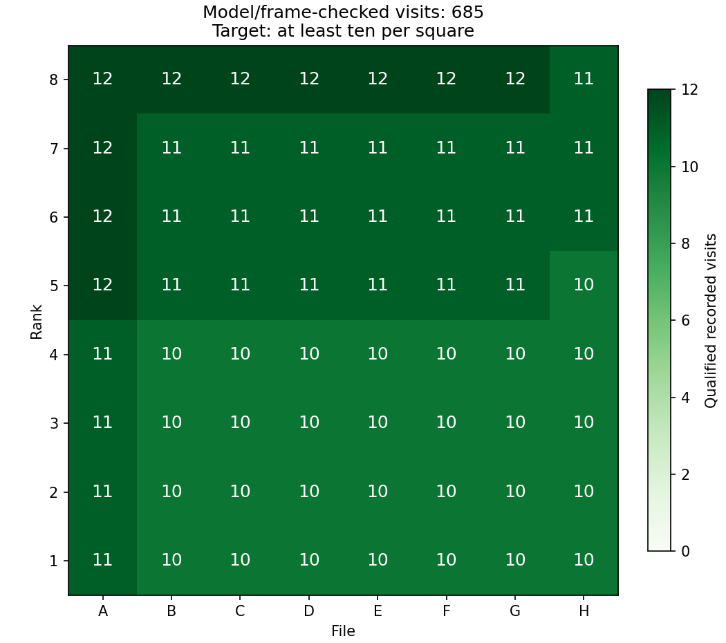
The repeated collector uses a closed adjacent-square circuit and alternates direction. It retains unsuccessful primary moves and permits one bounded correction after a known completed command. Faults, unknown writes, failed corrections and recording errors stop the batch. Neither USB nor camera ownership changes.
The first repeated circuit stopped before dispatching A6. Its packet-rate bound covered measured joints but omitted the cached command targets used by the native executor. Native receipts confirm zero motor writes for that A6 command. The calculation now covers both starts and has a regression test. After I explicitly inspected the bench, the native inspection helper archived the original Stop unchanged, with zero motor commands.
A later G7 correction completed natively but failed the modeled arrival band. Its held-posture solution was only 18.07 mm high, leaving little margin above the 18 mm floor. That batch ended. The correction planner now requires 20–21.5 mm reference height, or solves a bounded 21 mm correction. A new recorded canary passed before collection continued; the original miss remains in the dataset.
A later A6 correction was rejected before submission by the unchanged 28 mm command-height ceiling. Candidate selection now applies that screen before ranking solutions. Its original primary miss remains recorded, and a new canary passed.
A subsequent G7 correction overshot horizontally by 5.35 mm after native completion. The batch ended, and a separate recorded canary preceded the remaining visits. These failures show why native completion alone is insufficient for the dataset label.
Six complete 64-square panels passed, alongside the retained canaries and split circuits. Completed full-panel times ranged from 94.03 to 119.96 seconds, including corrections and all gaps. These are collection times, not half-second leg qualifications.
The new evidence archive contains 37 camera/joint captures, including interrupted attempts, with zero dropped rows/events or writer errors and a checksum-verified copy on a separate drive. Private bench images remain private. Download the board coverage and per-visit metrics, archive verification, and the zero-write reconciliation, the inspected recovery, and the later G7 miss.
Castor is idle after targeting A1 at the end of collection. The current deterministic controller is sufficient to collect this dataset; a neural network is not required for the geometric motion calculation.
I also staged the current code on Pollux, the second arm on Epimetheus. All 85 Python tests and both C++ checks pass there. Its wrist fisheye is connected, but its fixed C270 is absent; its own joint limits and 20 mm board routes remain unqualified. Its Stop stays preserved, and no collection motion has been sent. Castor’s calibration and ticks cannot be copied onto Pollux. Pollux readiness audit.